Study Overview
This collection of notebooks surrounds a diary study that I assisted with. Diary studies are longitudinal studies in which participants routinely complete surveys throughout. These are especially useful for tracking things such as mood, exercise/diet habits, and for our intents and purposes, social media usage.
In this notebook, I’ll be walking through the process of converting the raw data from wide to long format. All of the accompanying datasets can be found here.
In the initial survey (day 0), participants were asked to give several different types of ratings for 6 social media platforms: Facebook, Youtube, Snapchat, Instagram, Twitter, and Pinterest. Aside from the IBIS measure, several ubiquitous market research measures were used:
- Purchase Intention (“_use”)
- Overall opinion (“_op”)
- Likelihood to recomment (“_rec”)
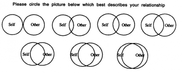
The IBIS measure is adapted from the Inclusion of Others in Self (IOS) scale, originally developed as a way to measure to measure intimacy. Individuals are simply asked about their relationship with a partner and shown a series of increasingly overlapping circles - the idea being that more overlap will indicate stronger relationships.
Adaptation of this measure was originally proposed following the rise in the theoretical perspective of brand relationships, or the notion that individuals develop relationships with brands similarly to ones formed with other people. The bulk of the work concerning this measure had been mostly conceptual, and to date, our study would be the first using actual usage data.
We had 2 main questions:
- Does IBIS prospectively predict usage?
- If so, how does it perform relative to other widely used measures?
Day 0 Transformation
First, we’ll need to import the libraries that we will need. The “set_option” parameters are there to make viewing all of the columns easier.
There were several components to the overall experiment, and this current cleaning/analysis will focus on social media platforms.
import numpy as np
import pandas as pd
pd.set_option('display.max_rows', 500)
pd.set_option('display.max_columns', 500)
pd.set_option('display.width', 1000)
Let’s take a look at the data.
day_zero = pd.read_csv('day_zero.csv')

day_zero.head()
| Unnamed: 0 | age | ethnicity | gender | fsc_1 | fsc_2 | fsc_3 | fsc_4 | aquafina_percep | dasani_percep | fiji_percep | starbucks_percep | coffee_bean_percep | dunkin_donuts_percep | freudian_sip_percep | twitter_percep | snapchat_percep | youtube_percep | coke_percep | sprite_percep | pepsi_percep | budweiser_percep | miller_lite_percep | corona_percep | blue_moon_percep | coors_percep | facebook_percep | instagram_percep | pinterest_percep | coke_percep.1 | sprite_percep.1 | pepsi_percep.1 | budweiser_percep.1 | miller_lite_percep.1 | corona_percep.1 | blue_moon_percep.1 | coors_percep.1 | facebook_percep.1 | instagram_percep.1 | pinterest_percep.1 | aquafina_percep.1 | dasani_percep.1 | fiji_percep.1 | starbucks_percep.1 | coffee_bean_percep.1 | dunkin_donuts_percep.1 | freudian_sip_percep.1 | twitter_percep.1 | snapchat_percep.1 | youtube_percep.1 | corona_buy | blue_moon_buy | aquafina_buy | dasani_buy | fiji_buy | starbucks_buy | coffee_bean_buy | dunkin_donuts_buy | freudian_sip_buy | coke_buy | sprite_buy | pepsi_buy | budweiser_buy | coors_buy | miller_lite_buy | coke_buy.1 | sprite_buy.1 | pepsi_buy.1 | budweiser_buy.1 | coors_buy.1 | miller_lite_buy.1 | corona_buy.1 | blue_moon_buy.1 | aquafina_buy.1 | dasani_buy.1 | fiji_buy.1 | starbucks_buy.1 | coffee_bean_buy.1 | dunkin_donuts_buy.1 | freudian_sip_buy.1 | facebook_use | youtube_use | snapchat_use | twitter_use | instagram_use | pinterest_use | pinterest_use.1 | instagram_use.1 | twitter_use.1 | snapchat_use.1 | youtube_use.1 | facebook_use.1 | corona_rec | blue_moon_rec | aquafina_rec | dasani_rec | fiji_rec | starbucks_rec | coffee_bean_rec | dunkin_donuts_rec | freudian_sip_rec | coke_rec | sprite_rec | pepsi_rec | budweiser_rec | coors_rec | miller_lite_rec | facebook_rec | youtube_rec | snapchat_rec | twitter_rec | instagram_rec | pinterest_rec | pinterest_rec.1 | instagram_rec.1 | twitter_rec.1 | snapchat_rec.1 | youtube_rec.1 | facebook_rec.1 | miller_lite_rec.1 | coors_rec.1 | budweiser_rec.1 | pepsi_rec.1 | sprite_rec.1 | coke_rec.1 | freudian_sip_rec.1 | dunkin_donuts_rec.1 | coffee_bean_rec.1 | starbucks_rec.1 | fiji_rec.1 | dasani_rec.1 | aquafina_rec.1 | blue_moon_rec.1 | corona_rec.1 | corono_op | blue_moon_op | aquafina_op | dasani_op | fiji_op | starbucks_op | coffee_bean_op | dunkin_donuts_op | freudian_sip_op | coke_op | sprite_op | pepsi_op | budweiser_op | coors_op | miller_lite_op | facebook_op | youtube_op | snapchat_op | instagram_op | twitter_op | pinterest_op | pinterest_op.1 | instagram_op.1 | twitter_op.1 | snapchat_op.1 | youtube_op.1 | facebook_op.1 | miller_lite_op.1 | coors_op.1 | budweiser_op.1 | pepsi_op.1 | sprite_op.1 | coke_op.1 | freudian_sip_op.1 | dunkin_donuts_op.1 | coffee_bean_op.1 | starbucks_op.1 | fiji_op.1 | dasani_op.1 | aquafina_op.1 | blue_moon_op.1 | corona_op | pos_1 | pos_2 | pos_3 | pos_4 | pos_5 | neg_1 | neg_2 | neg_3 | neg_4 | neg_5 | neg_6 | neg_7 | neg_8 | participant | |
|---|---|---|---|---|---|---|---|---|---|---|---|---|---|---|---|---|---|---|---|---|---|---|---|---|---|---|---|---|---|---|---|---|---|---|---|---|---|---|---|---|---|---|---|---|---|---|---|---|---|---|---|---|---|---|---|---|---|---|---|---|---|---|---|---|---|---|---|---|---|---|---|---|---|---|---|---|---|---|---|---|---|---|---|---|---|---|---|---|---|---|---|---|---|---|---|---|---|---|---|---|---|---|---|---|---|---|---|---|---|---|---|---|---|---|---|---|---|---|---|---|---|---|---|---|---|---|---|---|---|---|---|---|---|---|---|---|---|---|---|---|---|---|---|---|---|---|---|---|---|---|---|---|---|---|---|---|---|---|---|---|---|---|---|---|---|---|---|---|---|---|---|---|---|---|---|---|---|---|---|---|---|---|---|---|---|---|---|---|---|---|
| 0 | 0 | 18 | 1 | 1 | 3 | 3 | 2 | 2 | NaN | NaN | NaN | NaN | NaN | NaN | NaN | NaN | NaN | NaN | NaN | NaN | NaN | NaN | NaN | NaN | NaN | NaN | NaN | NaN | NaN | 4.0 | 3.0 | 3.0 | 1.0 | 1.0 | 1.0 | 1.0 | 1.0 | 4.0 | 7.0 | 3.0 | 3.0 | 4.0 | 3.0 | 4.0 | 4.0 | 5.0 | 3.0 | 4.0 | 7.0 | 7.0 | 5.0 | 5.0 | 2.0 | 2.0 | 3.0 | 2.0 | 2.0 | 3.0 | 2.0 | 2.0 | 2.0 | 2.0 | 5.0 | 5.0 | 5.0 | NaN | NaN | NaN | NaN | NaN | NaN | NaN | NaN | NaN | NaN | NaN | NaN | NaN | NaN | NaN | NaN | NaN | NaN | NaN | NaN | NaN | 2.0 | 1.0 | 5.0 | 1.0 | 1.0 | 1.0 | 6.0 | 6.0 | 4.0 | 4.0 | 4.0 | 3.0 | 3.0 | 3.0 | 3.0 | 3.0 | 3.0 | 3.0 | 6.0 | 6.0 | 6.0 | 3.0 | 1.0 | 1.0 | 2.0 | 1.0 | 2.0 | NaN | NaN | NaN | NaN | NaN | NaN | NaN | NaN | NaN | NaN | NaN | NaN | NaN | NaN | NaN | NaN | NaN | NaN | NaN | NaN | NaN | NaN | NaN | NaN | NaN | NaN | NaN | NaN | NaN | NaN | NaN | NaN | NaN | NaN | NaN | NaN | NaN | NaN | NaN | NaN | NaN | NaN | 2.0 | 1.0 | 1.0 | 1.0 | 1.0 | 1.0 | 3.0 | 3.0 | 3.0 | 2.0 | 1.0 | 2.0 | 2.0 | 1.0 | 2.0 | 2.0 | 4.0 | 3.0 | 3.0 | 3.0 | 3.0 | 1 | 3 | 3 | 5 | 3 | 3 | 2 | 3 | 3 | 2 | 2 | 2 | 1 | 0 |
| 1 | 1 | 18 | 1 | 2 | 3 | 2 | 2 | 2 | NaN | NaN | NaN | NaN | NaN | NaN | NaN | NaN | NaN | NaN | NaN | NaN | NaN | NaN | NaN | NaN | NaN | NaN | NaN | NaN | NaN | 1.0 | 4.0 | 1.0 | 1.0 | 1.0 | 1.0 | 1.0 | 1.0 | 1.0 | 7.0 | 1.0 | 2.0 | 1.0 | 2.0 | 4.0 | 2.0 | 2.0 | 3.0 | 1.0 | 7.0 | 7.0 | NaN | NaN | NaN | NaN | NaN | NaN | NaN | NaN | NaN | NaN | NaN | NaN | NaN | NaN | NaN | 4.0 | 3.0 | 4.0 | 5.0 | 5.0 | 5.0 | 5.0 | 5.0 | 3.0 | 3.0 | 4.0 | 3.0 | 3.0 | 4.0 | 2.0 | 5.0 | 2.0 | 1.0 | 6.0 | 1.0 | 6.0 | NaN | NaN | NaN | NaN | NaN | NaN | 7.0 | 7.0 | 3.0 | 4.0 | 3.0 | 2.0 | 2.0 | 2.0 | 3.0 | 5.0 | 2.0 | 5.0 | 7.0 | 7.0 | 7.0 | 5.0 | 2.0 | 2.0 | 5.0 | 2.0 | 6.0 | NaN | NaN | NaN | NaN | NaN | NaN | NaN | NaN | NaN | NaN | NaN | NaN | NaN | NaN | NaN | NaN | NaN | NaN | NaN | NaN | NaN | 3.0 | 3.0 | 2.0 | 3.0 | 2.0 | 2.0 | 2.0 | 2.0 | 2.0 | 4.0 | 2.0 | 4.0 | 3.0 | 3.0 | 3.0 | 3.0 | 2.0 | 2.0 | 2.0 | 2.0 | 3.0 | NaN | NaN | NaN | NaN | NaN | NaN | NaN | NaN | NaN | NaN | NaN | NaN | NaN | NaN | NaN | NaN | NaN | NaN | NaN | NaN | NaN | 1 | 1 | 9 | 1 | 1 | 1 | 1 | 4 | 1 | 3 | 1 | 1 | 1 | 1 |
| 2 | 2 | 18 | 6 | 2 | 5 | 5 | 1 | 1 | NaN | NaN | NaN | NaN | NaN | NaN | NaN | NaN | NaN | NaN | NaN | NaN | NaN | NaN | NaN | NaN | NaN | NaN | NaN | NaN | NaN | 1.0 | 2.0 | 1.0 | 1.0 | 1.0 | 1.0 | 1.0 | 1.0 | 2.0 | 5.0 | 1.0 | 5.0 | 6.0 | 4.0 | 1.0 | 4.0 | 1.0 | 6.0 | 6.0 | 4.0 | 5.0 | NaN | NaN | NaN | NaN | NaN | NaN | NaN | NaN | NaN | NaN | NaN | NaN | NaN | NaN | NaN | 5.0 | 4.0 | 5.0 | 5.0 | 5.0 | 5.0 | 5.0 | 5.0 | 1.0 | 2.0 | 3.0 | 5.0 | 2.0 | 5.0 | 1.0 | NaN | NaN | NaN | NaN | NaN | NaN | 6.0 | 1.0 | 1.0 | 1.0 | 1.0 | 2.0 | 7.0 | 7.0 | 1.0 | 1.0 | 1.0 | 7.0 | 1.0 | 7.0 | 2.0 | 7.0 | 6.0 | 7.0 | 7.0 | 7.0 | 7.0 | 4.0 | 1.0 | 1.0 | 1.0 | 1.0 | 5.0 | NaN | NaN | NaN | NaN | NaN | NaN | NaN | NaN | NaN | NaN | NaN | NaN | NaN | NaN | NaN | NaN | NaN | NaN | NaN | NaN | NaN | NaN | NaN | NaN | NaN | NaN | NaN | NaN | NaN | NaN | NaN | NaN | NaN | NaN | NaN | NaN | NaN | NaN | NaN | NaN | NaN | NaN | 3.0 | 1.0 | 1.0 | 2.0 | 1.0 | 2.0 | 5.0 | 5.0 | 5.0 | 5.0 | 4.0 | 5.0 | 2.0 | 5.0 | 1.0 | 5.0 | 1.0 | 1.0 | 1.0 | 5.0 | 5.0 | 1 | 1 | 1 | 1 | 1 | 1 | 1 | 1 | 1 | 1 | 1 | 1 | 1 | 2 |
| 3 | 3 | 18 | 5 | 1 | 7 | 2 | 1 | 4 | 3.0 | 3.0 | 3.0 | 1.0 | 1.0 | 1.0 | 4.0 | 4.0 | 5.0 | 7.0 | 1.0 | 1.0 | 1.0 | 1.0 | 1.0 | 1.0 | 1.0 | 1.0 | 1.0 | 4.0 | 1.0 | NaN | NaN | NaN | NaN | NaN | NaN | NaN | NaN | NaN | NaN | NaN | NaN | NaN | NaN | NaN | NaN | NaN | NaN | NaN | NaN | NaN | NaN | NaN | NaN | NaN | NaN | NaN | NaN | NaN | NaN | NaN | NaN | NaN | NaN | NaN | NaN | 5.0 | 5.0 | 5.0 | 5.0 | 5.0 | 5.0 | 5.0 | 5.0 | 3.0 | 3.0 | 3.0 | 5.0 | 5.0 | 5.0 | 2.0 | NaN | NaN | NaN | NaN | NaN | NaN | 6.0 | 3.0 | 4.0 | 1.0 | 1.0 | 6.0 | 7.0 | 7.0 | 4.0 | 4.0 | 4.0 | 7.0 | 7.0 | 3.0 | 2.0 | 7.0 | 7.0 | 7.0 | 7.0 | 7.0 | 7.0 | 7.0 | 1.0 | 3.0 | 2.0 | 4.0 | 7.0 | NaN | NaN | NaN | NaN | NaN | NaN | NaN | NaN | NaN | NaN | NaN | NaN | NaN | NaN | NaN | NaN | NaN | NaN | NaN | NaN | NaN | 4.0 | 3.0 | 3.0 | 3.0 | 3.0 | 3.0 | 3.0 | 2.0 | 2.0 | 5.0 | 5.0 | 5.0 | 3.0 | 3.0 | 3.0 | 5.0 | 4.0 | 4.0 | 3.0 | 2.0 | 3.0 | NaN | NaN | NaN | NaN | NaN | NaN | NaN | NaN | NaN | NaN | NaN | NaN | NaN | NaN | NaN | NaN | NaN | NaN | NaN | NaN | NaN | 7 | 6 | 9 | 6 | 1 | 3 | 1 | 1 | 1 | 1 | 1 | 1 | 1 | 3 |
| 4 | 4 | 18 | 4 | 1 | 4 | 1 | 3 | 2 | NaN | NaN | NaN | NaN | NaN | NaN | NaN | NaN | NaN | NaN | NaN | NaN | NaN | NaN | NaN | NaN | NaN | NaN | NaN | NaN | NaN | 4.0 | 3.0 | 2.0 | 1.0 | 1.0 | 1.0 | 1.0 | 1.0 | 3.0 | 7.0 | 1.0 | 3.0 | 4.0 | 3.0 | 6.0 | 4.0 | 4.0 | 4.0 | 3.0 | 5.0 | 7.0 | 4.0 | 4.0 | 3.0 | 3.0 | 2.0 | 1.0 | 2.0 | 3.0 | 3.0 | 4.0 | 3.0 | 3.0 | 4.0 | 4.0 | 4.0 | NaN | NaN | NaN | NaN | NaN | NaN | NaN | NaN | NaN | NaN | NaN | NaN | NaN | NaN | NaN | 4.0 | 1.0 | 1.0 | 3.0 | 1.0 | 5.0 | NaN | NaN | NaN | NaN | NaN | NaN | 7.0 | 7.0 | 3.0 | 3.0 | 3.0 | 1.0 | 2.0 | 3.0 | 1.0 | 3.0 | 2.0 | 3.0 | 7.0 | 7.0 | 7.0 | 3.0 | 3.0 | 1.0 | 1.0 | 1.0 | 5.0 | NaN | NaN | NaN | NaN | NaN | NaN | NaN | NaN | NaN | NaN | NaN | NaN | NaN | NaN | NaN | NaN | NaN | NaN | NaN | NaN | NaN | NaN | NaN | NaN | NaN | NaN | NaN | NaN | NaN | NaN | NaN | NaN | NaN | NaN | NaN | NaN | NaN | NaN | NaN | NaN | NaN | NaN | 3.0 | 2.0 | 2.0 | 2.0 | 3.0 | 3.0 | 4.0 | 4.0 | 4.0 | 2.0 | 2.0 | 3.0 | 1.0 | 2.0 | 3.0 | 1.0 | 1.0 | 2.0 | 3.0 | 4.0 | 4.0 | 3 | 6 | 8 | 6 | 7 | 2 | 6 | 1 | 4 | 2 | 3 | 6 | 1 | 4 |
Now, we need to grab the relevant social media columns.
#Getting social media columns and sorting
sm_cols = [col for col in day_zero if 'participant' in col or 'facebook' in col
          or 'youtube' in col or 'snapchat' in col or 'instagram' in col
          or 'twitter' in col or 'pinterest' in col]
sm_cols.sort()

day_zero_sm = day_zero[sm_cols]
day_zero_sm.head()
| facebook_op | facebook_op.1 | facebook_percep | facebook_percep.1 | facebook_rec | facebook_rec.1 | facebook_use | facebook_use.1 | instagram_op | instagram_op.1 | instagram_percep | instagram_percep.1 | instagram_rec | instagram_rec.1 | instagram_use | instagram_use.1 | participant | pinterest_op | pinterest_op.1 | pinterest_percep | pinterest_percep.1 | pinterest_rec | pinterest_rec.1 | pinterest_use | pinterest_use.1 | snapchat_op | snapchat_op.1 | snapchat_percep | snapchat_percep.1 | snapchat_rec | snapchat_rec.1 | snapchat_use | snapchat_use.1 | twitter_op | twitter_op.1 | twitter_percep | twitter_percep.1 | twitter_rec | twitter_rec.1 | twitter_use | twitter_use.1 | youtube_op | youtube_op.1 | youtube_percep | youtube_percep.1 | youtube_rec | youtube_rec.1 | youtube_use | youtube_use.1 | |
|---|---|---|---|---|---|---|---|---|---|---|---|---|---|---|---|---|---|---|---|---|---|---|---|---|---|---|---|---|---|---|---|---|---|---|---|---|---|---|---|---|---|---|---|---|---|---|---|---|---|
| 0 | NaN | 1.0 | NaN | 4.0 | 3.0 | NaN | NaN | 1.0 | NaN | 1.0 | NaN | 7.0 | 1.0 | NaN | NaN | 1.0 | 0 | NaN | 2.0 | NaN | 3.0 | 2.0 | NaN | NaN | 2.0 | NaN | 1.0 | NaN | 7.0 | 1.0 | NaN | NaN | 1.0 | NaN | 1.0 | NaN | 4.0 | 2.0 | NaN | NaN | 5.0 | NaN | 1.0 | NaN | 7.0 | 1.0 | NaN | NaN | 1.0 |
| 1 | 3.0 | NaN | NaN | 1.0 | 5.0 | NaN | 5.0 | NaN | 2.0 | NaN | NaN | 7.0 | 2.0 | NaN | 1.0 | NaN | 1 | 3.0 | NaN | NaN | 1.0 | 6.0 | NaN | 6.0 | NaN | 2.0 | NaN | NaN | 7.0 | 2.0 | NaN | 1.0 | NaN | 2.0 | NaN | NaN | 1.0 | 5.0 | NaN | 6.0 | NaN | 2.0 | NaN | NaN | 7.0 | 2.0 | NaN | 2.0 | NaN |
| 2 | NaN | 2.0 | NaN | 2.0 | 4.0 | NaN | NaN | 2.0 | NaN | 1.0 | NaN | 5.0 | 1.0 | NaN | NaN | 1.0 | 2 | NaN | 3.0 | NaN | 1.0 | 5.0 | NaN | NaN | 6.0 | NaN | 2.0 | NaN | 4.0 | 1.0 | NaN | NaN | 1.0 | NaN | 1.0 | NaN | 6.0 | 1.0 | NaN | NaN | 1.0 | NaN | 1.0 | NaN | 5.0 | 1.0 | NaN | NaN | 1.0 |
| 3 | 5.0 | NaN | 1.0 | NaN | 7.0 | NaN | NaN | 6.0 | 3.0 | NaN | 4.0 | NaN | 4.0 | NaN | NaN | 3.0 | 3 | 3.0 | NaN | 1.0 | NaN | 7.0 | NaN | NaN | 6.0 | 4.0 | NaN | 5.0 | NaN | 3.0 | NaN | NaN | 1.0 | 2.0 | NaN | 4.0 | NaN | 2.0 | NaN | NaN | 4.0 | 4.0 | NaN | 7.0 | NaN | 1.0 | NaN | NaN | 1.0 |
| 4 | NaN | 3.0 | NaN | 3.0 | 3.0 | NaN | 4.0 | NaN | NaN | 2.0 | NaN | 7.0 | 1.0 | NaN | 1.0 | NaN | 4 | NaN | 3.0 | NaN | 1.0 | 5.0 | NaN | 5.0 | NaN | NaN | 2.0 | NaN | 5.0 | 1.0 | NaN | 1.0 | NaN | NaN | 2.0 | NaN | 3.0 | 1.0 | NaN | 3.0 | NaN | NaN | 3.0 | NaN | 7.0 | 3.0 | NaN | 1.0 | NaN |
Brand/platform ratings were counterbalanced, which is why there are so many missing values. To simplify the columns for analysis, I’ll simply fill the NAs with 0s and add each respective platform’s columns together.
platforms = ['facebook', 'youtube', 'snapchat', 'instagram', 'twitter', 'pinterest']
measures = ['op', 'percep', 'rec', 'use']

for platform in platforms:
    for measure in measures:
        day_zero_sm[f'{platform}_{measure}_final'] = (
        day_zero_sm.filter(like = platform)
         .filter(like = measure)
         .sum(axis = 1)
        )
#Filtering and renaming 'final' columns
day_zero_sm_fin = day_zero_sm[[col for col in day_zero_sm.columns if '_final' in col
                              or 'participant' in col]]
day_zero_sm_fin.columns = day_zero_sm_fin.columns.str.rstrip('_final')
day_zero_sm_fin.head()
| participant | facebook_op | facebook_percep | facebook_rec | facebook_use | youtube_op | youtube_percep | youtube_rec | youtube_use | snapchat_op | snapchat_percep | snapchat_rec | snapchat_use | instagram_op | instagram_percep | instagram_rec | instagram_use | twitter_op | twitter_percep | twitter_rec | twitter_use | pinterest_op | pinterest_percep | pinterest_rec | pinterest_use | |
|---|---|---|---|---|---|---|---|---|---|---|---|---|---|---|---|---|---|---|---|---|---|---|---|---|---|
| 0 | 0 | 1.0 | 4.0 | 3.0 | 1.0 | 1.0 | 7.0 | 1.0 | 1.0 | 1.0 | 7.0 | 1.0 | 1.0 | 1.0 | 7.0 | 1.0 | 1.0 | 1.0 | 4.0 | 2.0 | 5.0 | 2.0 | 3.0 | 2.0 | 2.0 |
| 1 | 1 | 3.0 | 1.0 | 5.0 | 5.0 | 2.0 | 7.0 | 2.0 | 2.0 | 2.0 | 7.0 | 2.0 | 1.0 | 2.0 | 7.0 | 2.0 | 1.0 | 2.0 | 1.0 | 5.0 | 6.0 | 3.0 | 1.0 | 6.0 | 6.0 |
| 2 | 2 | 2.0 | 2.0 | 4.0 | 2.0 | 1.0 | 5.0 | 1.0 | 1.0 | 2.0 | 4.0 | 1.0 | 1.0 | 1.0 | 5.0 | 1.0 | 1.0 | 1.0 | 6.0 | 1.0 | 1.0 | 3.0 | 1.0 | 5.0 | 6.0 |
| 3 | 3 | 5.0 | 1.0 | 7.0 | 6.0 | 4.0 | 7.0 | 1.0 | 1.0 | 4.0 | 5.0 | 3.0 | 1.0 | 3.0 | 4.0 | 4.0 | 3.0 | 2.0 | 4.0 | 2.0 | 4.0 | 3.0 | 1.0 | 7.0 | 6.0 |
| 4 | 4 | 3.0 | 3.0 | 3.0 | 4.0 | 3.0 | 7.0 | 3.0 | 1.0 | 2.0 | 5.0 | 1.0 | 1.0 | 2.0 | 7.0 | 1.0 | 1.0 | 2.0 | 3.0 | 1.0 | 3.0 | 3.0 | 1.0 | 5.0 | 5.0 |
df_dict = {}

for platform in platforms:
    #New df for each platform
    df_dict[platform] = day_zero_sm_fin[['participant',*[col for col in day_zero_sm_fin.columns
                                                     if platform in col]]]
    #Adding in platform name column for eventual long-form
    df_dict[platform]['platform'] = platform
    #Standardizing column names for just measure
    df_dict[platform].columns = [col.split('_')[-1] for col in df_dict[platform].columns]
day_zero_master = pd.concat([df_dict[k] for k,v in df_dict.items()])
Now that the data are in long-form, each participant should have 6 entries (i.e., 1 entry per platform). Let’s do a quick sanity check.
day_zero_master.sort_values('participant').head(12)
| participant | op | percep | rec | use | platform | |
|---|---|---|---|---|---|---|
| 0 | 0 | 1.0 | 4.0 | 3.0 | 1.0 | |
| 0 | 0 | 1.0 | 7.0 | 1.0 | 1.0 | snapchat |
| 0 | 0 | 1.0 | 7.0 | 1.0 | 1.0 | youtube |
| 0 | 0 | 2.0 | 3.0 | 2.0 | 2.0 | |
| 0 | 0 | 1.0 | 4.0 | 2.0 | 5.0 | |
| 0 | 0 | 1.0 | 7.0 | 1.0 | 1.0 | |
| 1 | 1 | 3.0 | 1.0 | 6.0 | 6.0 | |
| 1 | 1 | 3.0 | 1.0 | 5.0 | 5.0 | |
| 1 | 1 | 2.0 | 7.0 | 2.0 | 1.0 | snapchat |
| 1 | 1 | 2.0 | 7.0 | 2.0 | 1.0 | |
| 1 | 1 | 2.0 | 7.0 | 2.0 | 2.0 | youtube |
| 1 | 1 | 2.0 | 1.0 | 5.0 | 6.0 |
Next, we bring in the weekly survey data. We’ll need to make the same long-form transformations before we merge them to the initial survey.
Weekly Survey Transformations
wk_one = pd.read_csv('week_one.csv')
wk_two = pd.read_csv('week_two.csv')
wk_three= pd.read_csv('week_three.csv')

wk_one.head()
| Unnamed: 0 | coke | sprite | pepsi | other_soda | bud | coors | miller_lite | corona | blue_moon | other_beer | other_alcohol | aquafina | dasani | fiji | other_water | starbucks | coffee_bean | dunkin_donuts | freudian_sip | other_coffee | snapchat | youtube | participant | |||||
|---|---|---|---|---|---|---|---|---|---|---|---|---|---|---|---|---|---|---|---|---|---|---|---|---|---|---|---|---|
| 0 | 0 | 1 | 2 | 1 | 2 | 0 | 0 | 0 | 0.0 | 0 | 0 | 0 | 0 | 0 | 0 | 0 | 4 | 0 | 0 | 0 | 0 | 0.0 | 3.0 | 3.0 | 3.0 | 3.0 | 1 | 15 |
| 1 | 1 | 0 | 2 | 0 | 0 | 0 | 0 | 0 | 0.0 | 0 | 0 | 0 | 21 | 2 | 0 | 4 | 0 | 0 | 0 | 0 | 0 | 0.0 | 4.0 | 10.0 | 0.0 | 3.0 | 0 | 57 |
| 2 | 2 | 0 | 0 | 0 | 0 | 0 | 0 | 0 | 0.0 | 0 | 0 | 2 | 0 | 0 | 0 | 1 | 1 | 0 | 0 | 0 | 0 | 10.0 | 10.0 | 10.0 | 3.0 | 8.0 | 0 | 63 |
| 3 | 3 | 0 | 0 | 0 | 4 | 0 | 0 | 0 | 0.0 | 0 | 0 | 0 | 0 | 0 | 0 | 10 | 1 | 0 | 0 | 0 | 0 | 3.0 | 5.0 | 10.0 | 0.0 | 6.0 | 1 | 162 |
| 4 | 4 | 0 | 1 | 0 | 0 | 0 | 0 | 0 | 0.0 | 0 | 0 | 0 | 0 | 0 | 0 | 0 | 1 | 0 | 0 | 0 | 1 | 0.0 | 2.0 | 3.0 | 0.0 | 4.0 | 0 | 66 |
#Grabbing social media platforms
wk_dfs = [wk_one, wk_two, wk_three]

for i in range(len(wk_dfs)):
    wk_dfs[i] = wk_dfs[i][[col for col in wk_dfs[i] if 'participant' in col or 'facebook' in col
          or 'youtube' in col or 'snapchat' in col or 'instagram' in col
          or 'twitter' in col or 'pinterest' in col]]

    #Adding in a column for week #
    wk_dfs[i]['week'] = i+1

wk_dfs[0].head()
| snapchat | youtube | participant | week | |||||
|---|---|---|---|---|---|---|---|---|
| 0 | 0.0 | 3.0 | 3.0 | 3.0 | 3.0 | 1 | 15 | 1 |
| 1 | 0.0 | 4.0 | 10.0 | 0.0 | 3.0 | 0 | 57 | 1 |
| 2 | 10.0 | 10.0 | 10.0 | 3.0 | 8.0 | 0 | 63 | 1 |
| 3 | 3.0 | 5.0 | 10.0 | 0.0 | 6.0 | 1 | 162 | 1 |
| 4 | 0.0 | 2.0 | 3.0 | 0.0 | 4.0 | 0 | 66 | 1 |
To convert this to long-form, we’ll use the “melt” function.
Below is a brief demo of what each week’s df will look like, as well as the annotated code.
(
    wk_dfs[0].melt(
        #The values that we want to use as identifiers
        id_vars = ['participant', 'week'],

        #The columns that will unpivot - i.e., form 1 column where each participant will have
        #a row entry for each previous column. Since these are the only columns aside from
        #'participant' and 'week', we technically don't need to even state them, but this is
        #good to just see what's happening.
        value_vars = ['snapchat', 'instagram', 'facebook',
                        'youtube', 'twitter', 'pinterest'],

        #The name of the aforementioned new column - using "platform" to match the same column
        #named on the initial survey (so we can merge later)
        var_name = 'platform',

        #The name of the column for the values; here, the values being hours spent on that
        #platform for that week
        value_name = 'hrs_spent')
    .sort_values('participant')
    .head(12)
)
| participant | week | platform | hrs_spent | |
|---|---|---|---|---|
| 44 | 1 | 1 | snapchat | 8.0 |
| 314 | 1 | 1 | 1.0 | |
| 719 | 1 | 1 | 0.0 | |
| 449 | 1 | 1 | youtube | 5.0 |
| 584 | 1 | 1 | 0.0 | |
| 179 | 1 | 1 | 8.0 | |
| 744 | 2 | 1 | 0.0 | |
| 339 | 2 | 1 | 5.0 | |
| 204 | 2 | 1 | 10.0 | |
| 474 | 2 | 1 | youtube | 5.0 |
| 609 | 2 | 1 | 1.0 | |
| 69 | 2 | 1 | snapchat | 1.0 |
#Shortened melt code
for i in range(len(wk_dfs)):
    wk_dfs[i] = wk_dfs[i].melt(id_vars = ['participant', 'week'],
                              var_name = 'platform',
                              value_name = 'hrs_spent').sort_values('participant')
#Combining each melted week
weekly_long = pd.concat(wk_dfs).sort_values(['participant', 'week'])
#Sanity check: participant 1 should have 18 entries (6 for each week)
weekly_long.head(19)
| participant | week | platform | hrs_spent | |
|---|---|---|---|---|
| 44 | 1 | 1 | 0.0 | |
| 314 | 1 | 1 | youtube | 5.0 |
| 719 | 1 | 1 | 0.0 | |
| 449 | 1 | 1 | 1.0 | |
| 584 | 1 | 1 | 8.0 | |
| 179 | 1 | 1 | snapchat | 8.0 |
| 516 | 1 | 2 | 0.0 | |
| 812 | 1 | 2 | 0.0 | |
| 72 | 1 | 2 | 0.0 | |
| 664 | 1 | 2 | 10.0 | |
| 368 | 1 | 2 | youtube | 5.0 |
| 220 | 1 | 2 | snapchat | 6.0 |
| 638 | 1 | 3 | 6.0 | |
| 497 | 1 | 3 | 0.0 | |
| 779 | 1 | 3 | 0.0 | |
| 215 | 1 | 3 | snapchat | 8.0 |
| 356 | 1 | 3 | youtube | 10.0 |
| 74 | 1 | 3 | 0.0 | |
| 744 | 2 | 1 | 0.0 |
Things look good! All that’s left now is to merge the master weekly df to the initial.
Each participant will still have 6 entries per week, and their initial ratings that they gave each brand will be on that corresponding entry.
master = weekly_long.merge(day_zero_master)

master.head(18)
| participant | week | platform | hrs_spent | op | percep | rec | use | |
|---|---|---|---|---|---|---|---|---|
| 0 | 1 | 1 | 0.0 | 2.0 | 1.0 | 5.0 | 6.0 | |
| 1 | 1 | 2 | 0.0 | 2.0 | 1.0 | 5.0 | 6.0 | |
| 2 | 1 | 3 | 0.0 | 2.0 | 1.0 | 5.0 | 6.0 | |
| 3 | 1 | 1 | youtube | 5.0 | 2.0 | 7.0 | 2.0 | 2.0 |
| 4 | 1 | 2 | youtube | 5.0 | 2.0 | 7.0 | 2.0 | 2.0 |
| 5 | 1 | 3 | youtube | 10.0 | 2.0 | 7.0 | 2.0 | 2.0 |
| 6 | 1 | 1 | 0.0 | 3.0 | 1.0 | 6.0 | 6.0 | |
| 7 | 1 | 2 | 0.0 | 3.0 | 1.0 | 6.0 | 6.0 | |
| 8 | 1 | 3 | 0.0 | 3.0 | 1.0 | 6.0 | 6.0 | |
| 9 | 1 | 1 | 1.0 | 3.0 | 1.0 | 5.0 | 5.0 | |
| 10 | 1 | 2 | 0.0 | 3.0 | 1.0 | 5.0 | 5.0 | |
| 11 | 1 | 3 | 0.0 | 3.0 | 1.0 | 5.0 | 5.0 | |
| 12 | 1 | 1 | 8.0 | 2.0 | 7.0 | 2.0 | 1.0 | |
| 13 | 1 | 2 | 10.0 | 2.0 | 7.0 | 2.0 | 1.0 | |
| 14 | 1 | 3 | 6.0 | 2.0 | 7.0 | 2.0 | 1.0 | |
| 15 | 1 | 1 | snapchat | 8.0 | 2.0 | 7.0 | 2.0 | 1.0 |
| 16 | 1 | 2 | snapchat | 6.0 | 2.0 | 7.0 | 2.0 | 1.0 |
| 17 | 1 | 3 | snapchat | 8.0 | 2.0 | 7.0 | 2.0 | 1.0 |
#master.to_csv('sm_master.csv')