Multilevel Modeling: A brief primer
The data are completely processed, and we’ve got a good idea of what’s going on in them. Now, we can get the exciting part! A full overview of multilevel linear modeling (MLM) is beyond the scope of this article, but I’ll give a short discussion on why this method of analysis was chosen.
MLM is used for analyses of data that have certain groupings, as well as data with repeated observations. In the present study, there are both. We have a set of different platforms, and each participant is also measured 3 times (weeks) for each platform. If we were to do a linear regressions, this structure inherently violates one of that model’s assumptions: independence of errors - i.e., that errors are uncorrelaed. In repeated measures observations, we’re going to have observations that are more alike than others since the same person is going to have multiple measurements! Additionally, as the EDA portion hinted at, there are going to be observations for certain platforms that are more alike than others. For example, instagram will, on average, have much more favorable ratings and higher usage than Pinterest. An advantage of MLM is that the assumption of independence of errrors does not have to be true.
In a standard linear regression, a single intercept value is estimated, which assumes a “one-size-fits-all” value. In MLM, we can estimate random intercepts for any differences in groupings. Take another look at the mean usages for each platform.
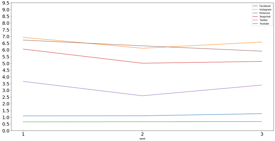
The variation in intercepts (where each platform hits the y-axis) is stark enough to illustrate that we should probably not estimate 1 intercept here. Random intercepts in MLM will be able to account for this. Similarly, we can look at participants’ average usage times for all apps each week.
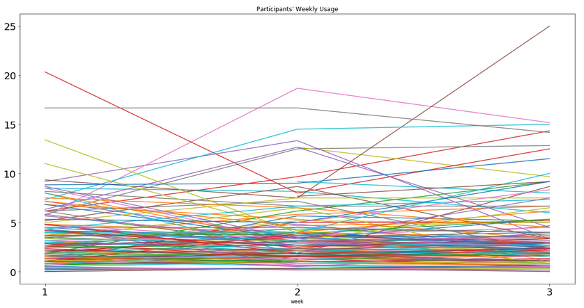
Using MLM, we will be able to estimate separate intercepts for each participant as well! By taking into account these differences, we will be able to get more accurate coefficients for our predictors since we remove differences associated with both individual participants as well as the platforms.
The actual modeling will follow these steps:
- Fixed intercept
- Random intercept - participants
- Random intercept - platforms
- Addition of predictors
Modeling
For the actual modeling, we’ll be using the lme4 library in R.
First, we need to import the data and necessary R packages.
library(lme4)
#For p-values of predictors
library(lmerTest)
#Import csv
library(readr)
#VIF
library(car)

data = read_csv('~sm_final.csv')

head(data)
## # A tibble: 6 x 9
##      X1 participant  week platform hrs_spent    op percep   rec   use
##   <dbl>       <dbl> <dbl> <chr>        <dbl> <dbl>  <dbl> <dbl> <dbl>
## 1     0           1     1 twitter          0     4      1     3     1
## 2     1           1     2 twitter          0     4      1     3     1
## 3     2           1     3 twitter          0     4      1     3     1
## 4     3           1     1 youtube          5     4      7     6     5
## 5     4           1     2 youtube          5     4      7     6     5
## 6     5           1     3 youtube         10     4      7     6     5
Fixed-intercept
We first fit a fixed intercept-only model to establish a baseline. When we compare models to see if random intercepts are justified, we need a way to quantify this. To do so, we will be doing chi-square difference tests. Each model will have an associated log-likelihood value; by subtracting our proposed model’s log-likelihood from the prior model, we can perform a chi-square test to check for significant differences. With a higher log-likelihood indicating greater model fit, a significant, positive chi-square difference justifies the new model. If this is confusing, we’ll set it in action in a moment.
First, we need to establish our baseline.
fixed_int <- lm(hrs_spent ~ 1, data)
summary(fixed_int)
##
## Call:
## lm(formula = hrs_spent ~ 1, data = data)
##
## Residuals:
##     Min      1Q  Median      3Q     Max
##  -3.678  -3.678  -2.678   1.322 108.322
##
## Coefficients:
##             Estimate Std. Error t value Pr(>|t|)
## (Intercept)   3.6782     0.1342   27.41   <2e-16 ***
## ---
## Signif. codes:  0 '***' 0.001 '**' 0.01 '*' 0.05 '.' 0.1 ' ' 1
##
## Residual standard error: 6.769 on 2543 degrees of freedom
Random-intercepts - Participants
Next, we add in our first random-intercepts.
rand_int_parts <- lmer(hrs_spent ~ (1 | participant), REML = FALSE, data)
summary(rand_int_parts)
## Linear mixed model fit by maximum likelihood . t-tests use
##   Satterthwaite's method [lmerModLmerTest]
## Formula: hrs_spent ~ (1 | participant)
##    Data: data
##
##      AIC      BIC   logLik deviance df.resid
##  16770.2  16787.7  -8382.1  16764.2     2541
##
## Scaled residuals:
##     Min      1Q  Median      3Q     Max
## -2.0251 -0.4606 -0.1977  0.2079 16.1312
##
## Random effects:
##  Groups      Name        Variance Std.Dev.
##  participant (Intercept)  6.323   2.515
##  Residual                39.410   6.278
## Number of obs: 2544, groups:  participant, 156
##
## Fixed effects:
##             Estimate Std. Error       df t value Pr(>|t|)
## (Intercept)   3.7013     0.2385 156.8496   15.52   <2e-16 ***
## ---
## Signif. codes:  0 '***' 0.001 '**' 0.01 '*' 0.05 '.' 0.1 ' ' 1
Something new we see in this output is the Random effects table. In the participants row, we get a variance score that we can use to examine the dependence of errors discussed above. We can do this by calculating the intraclass correlation (ICC), which will give us a value that measures how much of the variation in the data is due to - in our current case - participant differences.
We can manually calculate this by dividing the participant variance by the total variance: . In other words, 13.8% of the data’s variation is due to participant differences! This is not a ton, but it is not meaningless either.
To see if accounting for these differences is worthwhile, let’s compare the 2 models.
anova(rand_int_parts, fixed_int)
## Data: data
## Models:
## fixed_int: hrs_spent ~ 1
## rand_int_parts: hrs_spent ~ (1 | participant)
##                Df   AIC   BIC  logLik deviance  Chisq Chi Df Pr(>Chisq)
## fixed_int       2 16953 16965 -8474.4    16949
## rand_int_parts  3 16770 16788 -8382.1    16764 184.65      1  < 2.2e-16
##
## fixed_int
## rand_int_parts ***
## ---
## Signif. codes:  0 '***' 0.001 '**' 0.01 '*' 0.05 '.' 0.1 ' ' 1
We can see that there is an increase in log-likelihood of 184.65, and with p < 0.001, that this is significant. Our addition of random-intercepts for participants is justified.
Random-intercepts - Platforms
Now, we’ll add in random-intercepts for platforms. We will do so with participant intercepts still in the model since the previous test dictated their inclusion.
rand_int_parts_platforms <- lmer(hrs_spent ~ (1 | platform) + (1 | participant), REML = FALSE, data)
summary(rand_int_parts_platforms)
## Linear mixed model fit by maximum likelihood . t-tests use
##   Satterthwaite's method [lmerModLmerTest]
## Formula: hrs_spent ~ (1 | platform) + (1 | participant)
##    Data: data
##
##      AIC      BIC   logLik deviance df.resid
##  16447.3  16470.6  -8219.6  16439.3     2540
##
## Scaled residuals:
##     Min      1Q  Median      3Q     Max
## -2.3357 -0.4710 -0.1198  0.2157 16.8916
##
## Random effects:
##  Groups      Name        Variance Std.Dev.
##  participant (Intercept)  6.696   2.588
##  platform    (Intercept)  5.064   2.250
##  Residual                34.053   5.836
## Number of obs: 2544, groups:  participant, 156; platform, 6
##
## Fixed effects:
##             Estimate Std. Error     df t value Pr(>|t|)
## (Intercept)   3.7038     0.9493 6.6234   3.902  0.00656 **
## ---
## Signif. codes:  0 '***' 0.001 '**' 0.01 '*' 0.05 '.' 0.1 ' ' 1
We can calculate the ICC for platforms here as well: . So 11.1% of the variation in the data is due to platform differences, and together, participant and platform differences account for 25.7% of the total variation ()! These findings are in line with what we gathered from the visualizations and further demonstrate the strengths of MLM. We’ve accounted for what would have been a significant amount of noise in a typical linear regression.
Let’s validate that random-intercepts for platforms is indeed justified.
anova(rand_int_parts, rand_int_parts_platforms)
## Data: data
## Models:
## rand_int_parts: hrs_spent ~ (1 | participant)
## rand_int_parts_platforms: hrs_spent ~ (1 | platform) + (1 | participant)
##                          Df   AIC   BIC  logLik deviance  Chisq Chi Df
## rand_int_parts            3 16770 16788 -8382.1    16764
## rand_int_parts_platforms  4 16447 16471 -8219.6    16439 324.87      1
##                          Pr(>Chisq)
## rand_int_parts
## rand_int_parts_platforms  < 2.2e-16 ***
## ---
## Signif. codes:  0 '***' 0.001 '**' 0.01 '*' 0.05 '.' 0.1 ' ' 1
We can be comfortable with this addition, and now move onto adding our predictors.
Predictors
IBIS
We have our model that now accounts for differences between platforms and participants, and we can now examine our predictors. Our first research question was if IBIS significantly predicts social media usage. To examine this, we’ll model IBIS alone.
ibis_alone <- lmer(hrs_spent ~ percep + (1 | platform) + (1 | participant), REML = FALSE, data)
summary(ibis_alone)
## Linear mixed model fit by maximum likelihood . t-tests use
##   Satterthwaite's method [lmerModLmerTest]
## Formula: hrs_spent ~ percep + (1 | platform) + (1 | participant)
##    Data: data
##
##      AIC      BIC   logLik deviance df.resid
##  15916.1  15945.3  -7953.1  15906.1     2539
##
## Scaled residuals:
##     Min      1Q  Median      3Q     Max
## -2.4322 -0.4613 -0.0577  0.2564 17.8140
##
## Random effects:
##  Groups      Name        Variance Std.Dev.
##  participant (Intercept)  7.5536  2.7484
##  platform    (Intercept)  0.4752  0.6893
##  Residual                27.2958  5.2245
## Number of obs: 2544, groups:  participant, 156; platform, 6
##
## Fixed effects:
##               Estimate Std. Error         df t value Pr(>|t|)
## (Intercept)   -1.79416    0.43223   22.47869  -4.151 0.000402 ***
## percep         1.54934    0.06154 1277.00685  25.178  < 2e-16 ***
## ---
## Signif. codes:  0 '***' 0.001 '**' 0.01 '*' 0.05 '.' 0.1 ' ' 1
##
## Correlation of Fixed Effects:
##        (Intr)
## percep -0.506
Looking at the fixed effects table, we see that the coefficient for IBIS (i.e., percep) is 1.55 with, p < 0.001! We can interpret this as for each 1-unit increase in IBIS (for each increasing overlap chosen in the scale), weekly social media usage for that platform increases by 1.55 hours, and that this is significant.
Full Model
The second research question concerned IBIS’s performance relative to other popular measures. As we saw in the EDA portion, these measures do have moderate-strong correlations. We will use the variable inflation factor (VIF) to keep an eye on multicollinearity in the model. In short, VIF regresses each predictor on the others and returns a value. In general, a VIF > 10 is cause for concern.
Since the measures are on different scales (e.g., IBIS is 1-7, use intent is 1-6), we’ll also need to scale the variables. This changes the coefficient interpretations, so now instead a 1-unit increase, it will be a 1-standard deviation increase. This will allow us to directly compare the strength of each coefficient, though. Let’s fit the model!
full_model <- lmer(hrs_spent ~ scale(percep) + scale(use) + scale(op) + scale(rec) + (1 | platform) + (1 | participant), REML = FALSE, data)
summary(full_model)
## Linear mixed model fit by maximum likelihood . t-tests use
##   Satterthwaite's method [lmerModLmerTest]
## Formula:
## hrs_spent ~ scale(percep) + scale(use) + scale(op) + scale(rec) +
##     (1 | platform) + (1 | participant)
##    Data: data
##
##      AIC      BIC   logLik deviance df.resid
##  15775.6  15822.3  -7879.8  15759.6     2536
##
## Scaled residuals:
##     Min      1Q  Median      3Q     Max
## -2.2569 -0.4743 -0.0584  0.2974 18.0395
##
## Random effects:
##  Groups      Name        Variance Std.Dev.
##  participant (Intercept)  7.83926 2.7999
##  platform    (Intercept)  0.01642 0.1281
##  Residual                25.74848 5.0743
## Number of obs: 2544, groups:  participant, 156; platform, 6
##
## Fixed effects:
##                 Estimate Std. Error         df t value Pr(>|t|)
## (Intercept)      3.70754    0.25260   67.13862  14.677  < 2e-16 ***
## scale(percep)    1.57521    0.22177 1618.39977   7.103 1.82e-12 ***
## scale(use)       2.65324    0.20834  207.59806  12.735  < 2e-16 ***
## scale(op)        0.04564    0.16053 1505.63473   0.284    0.776
## scale(rec)      -0.20852    0.20655 2151.05756  -1.010    0.313
## ---
## Signif. codes:  0 '***' 0.001 '**' 0.01 '*' 0.05 '.' 0.1 ' ' 1
##
## Correlation of Fixed Effects:
##             (Intr) scl(pr) scl(s) scal(p)
## scale(prcp)  0.005
## scale(use)  -0.001 -0.597
## scale(op)   -0.001 -0.173   0.040
## scale(rec)  -0.004 -0.294  -0.271 -0.416
In this complete model, only IBIS and use intention are significant. Use intention is the clear winner, with a 1-SD increase indicating 2.65 greater hours of usage, while IBIS is associated with 1.58 hours. Importantly, these coefficients are controlling for the others. For a more complete interpretation of IBIS, we can say that accounting for differences between platforms and individuals, and while holding use intention, overall opinion, and likelihood to recommend constant, a 1-SD increase in IBIS is associated with 1.58 greater hours of platform usage.
vif(full_model)
## scale(percep)    scale(use)     scale(op)    scale(rec)
##      3.702163      3.250128      1.887815      3.018883
Looking at the VIF values, we can confirm that there is not a drastic amount of multicollinearity in the model either!
Conclusion
We did find evidence that IBIS does indeed predict social media usage. Although IBIS was outperformed by use intention, that it remained significant when controlling for all other predictors is impressive. Additionally, it outperformed 2 other common measures used in market research: overall opinion and likelihood to recommend.
IBIS is a single-item, easily administered scale. With preliminary evidence that it can prospectively predict social media usage, it does hold potential as an addition to studies where consumer behaviors are of interest.